Single-Layer Perceptron - Multiclass Classifier |Perceptron Learning Assignment Help

Import all necessary packages

# For Matrix and mathematical operations.
import numpy as np

# For visualizing graphs
import matplotlib
import matplotlib.pyplot as plt
%matplotlib inline

import seaborn as sns
from sklearn.metrics import classification_report, confusion_matrix
from sklearn import metrics

Data Preparation

X = np.array([
    [0, 0],
    [0, 1],
    [1, 0],
    [1, 1]])
​
y = np.array([0, 1, 2, 3])

def plot_multiclass_scatted_data(X, y):
    plt.style.use('ggplot')
    #plt.style.use(['dark_background'])
    #plt.style.use('classic')

    plot_colors = "rgby"
    class_names = "0123"
    cmap = plt.get_cmap('Paired')

    fig = plt.figure(figsize=(6, 6))
    x_min, x_max = X[:, 0].min() - 1, X[:, 0].max() + 1
    y_min, y_max = X[:, 1].min() - 1, X[:, 1].max() + 1

    # Plot the training points
    for i, n, c in zip(range(4), class_names, plot_colors):
        idx = np.where(y == i)
        plt.scatter(X[idx, 0], X[idx, 1], c=c, cmap=cmap, label="Class %s" % n)

    plt.xlim(x_min, x_max)
    plt.ylim(y_min, y_max)
    plt.legend(loc='upper right')
    plt.xlabel('x1')
    plt.ylabel('x2')
    plt.title('Multiclass Data Scatter Plot')

    plt.tight_layout()
    plt.show()

plot_multiclass_scatted_data(X, y)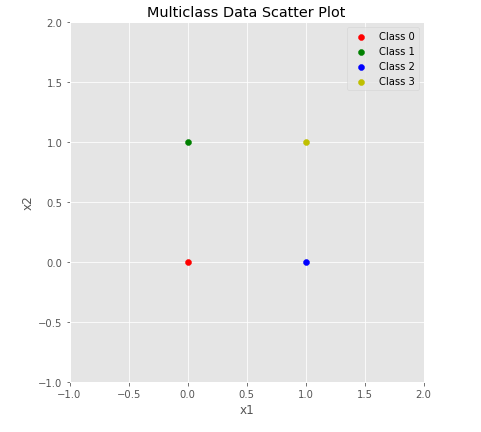

print("X shape ", X.shape)
print("y shape ", y.shape)

output:

X shape (4, 2) y shape (4,)

X_train = X.T

# Creating labels by one-hot encoding of y
digits = 4
examples = y.shape[0]
y_train = y.reshape(1, examples)
Y_train = np.eye(digits)[y_train.astype('int32')]
Y_train = Y_train.T.reshape(digits, examples)

print("X_train shape", X_train.shape)
print("Y_train shape", Y_train.shape)
print("X_train dataset\n ", X_train)
print("Y_train dataset\n", Y_train)

output:

X_train shape (2, 4) Y_train shape (4, 4)

X_train dataset [[0 0 1 1] [0 1 0 1]]

Y_train dataset [[1. 0. 0. 0.] [0. 1. 0. 0.] [0. 0. 1. 0.] [0. 0. 0. 1.]]

Neural Network Model Setup Step-by-step analysis of neural network outputs

# Neural Network Model
# initialization
np.random.seed(48)
n_features = X_train.shape[0]
n_out = Y_train.shape[0]
params = { "W": np.zeros((n_out, n_features)),
           "b": np.zeros((n_out, 1)) }
count=0

print("W shape", params["W"].shape)
print("b shape", params["b"].shape)

count+=1
learning_rate=1
cache = {}
cache["Z"] = np.dot(params["W"], X_train) + params["b"]
cache["P"] = softmax(cache["Z"])
cost = CrossEntropy(Y_train, cache["P"])
m_batch = X_train.shape[1]
dZ = (1./m_batch) * (cache["P"] - Y_train)  
dW =  np.dot(dZ, X_train.T)
db = np.sum(dZ, axis=1, keepdims=True)
  
print("Epoch", count)
print("X_train", X_train)
print("Z", cache["Z"])
print("P", cache["P"])
print("Cost {:.3f}".format(cost))
print("dZ", dZ)
print("dW", dW)
print("db", db)
print("W", params["W"])
print("b", params["b"])
params["W"] = params["W"] - learning_rate * dW
params["b"] = params["b"] - learning_rate * db
print("W*", params["W"])
print("b*", params["b"])

Neural Network Training

# Neural Network Model
# initialization
np.random.seed(48)
n_features = X_train.shape[0]
n_out = Y_train.shape[0]
params = { "W": np.zeros((n_out, n_features)),
           "b": np.zeros((n_out, 1)) }

# Hyper-parameters
learning_rate = 1
number_of_epoch=60
m_batch = X_train.shape[1]

# initially empty list, this will store all the training costs
costs = []  

# Start training
for epoch in range(number_of_epoch):
    
    cache = feed_forward(X_train, params)
    grads = back_propagate_softmax(X_train, Y_train, cache)
    params = update_parameters(params, grads, learning_rate)

    cost = CrossEntropy(Y_train, cache["P"])
    
    if (epoch % 1) == 0 or epoch == number_of_epoch - 1:
        print("Cost at epoch#{}: {:.3f}".format(epoch+1, cost))
        costs.append(cost)  

output:

Cost at epoch#1: 1.386
Cost at epoch#2: 1.269
Cost at epoch#3: 1.175
Cost at epoch#4: 1.094
Cost at epoch#5: 1.023
Cost at epoch#6: 0.959
Cost at epoch#7: 0.902
Cost at epoch#8: 0.850
Cost at epoch#9: 0.803
Cost at epoch#10: 0.760
Cost at epoch#11: 0.720
Cost at epoch#12: 0.684
Cost at epoch#13: 0.651
Cost at epoch#14: 0.620
Cost at epoch#15: 0.592
Cost at epoch#16: 0.566
Cost at epoch#17: 0.542
Cost at epoch#18: 0.520
Cost at epoch#19: 0.499
Cost at epoch#20: 0.479
Cost at epoch#21: 0.461
Cost at epoch#22: 0.444
Cost at epoch#23: 0.428
Cost at epoch#24: 0.413
...
...

Performance Evaluation

def plot_learning_curve(costs, learning_rate, total_epochs, save=False):
    
    # plot the cost
    plt.figure()
    #plt.style.use("fivethirtyeight")
    plt.style.use('seaborn-whitegrid')
    
    # the steps at with costs were recorded
    steps = int(total_epochs / len(costs))  
    plt.ylabel('Cost')
    plt.xlabel('Iterations ')
    plt.title("Learning rate =" + str(learning_rate))
    plt.plot(np.squeeze(costs))
    locs, labels = plt.xticks()
    # change x labels of the plot
    plt.xticks(locs[1:-1], tuple(np.array(locs[1:-1], dtype='int')*steps))  
    plt.xticks()
    if save:
        plt.savefig('Cost_Curve.png', bbox_inches='tight')
    plt.show()

plot_learning_curve(costs, learning_rate, 
                    number_of_epoch, save=True)

cache = feed_forward(X_train, params)
predictions = np.argmax(cache["P"], axis=0)
labels = np.argmax(Y_train, axis=0)
print("Input: \n", X_train)
print("Actual Output: \n ", Y_train)
print("Output Probabilities \n", cache["P"])
print("Labeled Output:           ", labels)
print("Predicted Output (argmax):", predictions)

def make_confusion_matrix(cf,
                          group_names=None,
                          categories='auto',
                          count=True,
                          percent=False,
                          cbar=True,
                          xyticks=True,
                          xyplotlabels=True,
                          sum_stats=True,
                          figsize=None,
                          cmap='Blues',
                          title=None):

    # CODE TO GENERATE TEXT INSIDE EACH SQUARE
    blanks = ['' for i in range(cf.size)]

    if group_names and len(group_names)==cf.size:
        group_labels = ["{}\n".format(value) for value in group_names]
    else:
        group_labels = blanks

    if count:
        group_counts = ["{0:0.0f}\n".format(value) for value in cf.flatten()]
    else:
        group_counts = blanks

    if percent:
        group_percentages = ["{0:.2%}".format(value) for value in cf.flatten()/np.sum(cf)]
    else:
        group_percentages = blanks

    box_labels = [f"{v1}{v2}{v3}".strip() for v1, v2, v3 in zip(group_labels,group_counts,group_percentages)]
    box_labels = np.asarray(box_labels).reshape(cf.shape[0],cf.shape[1])


    # CODE TO GENERATE SUMMARY STATISTICS & TEXT FOR SUMMARY STATS
    if sum_stats:
        #Accuracy is sum of diagonal divided by total observations
        accuracy  = np.trace(cf) / float(np.sum(cf))

        #if it is a binary confusion matrix, show some more stats
        if len(cf)==2:
            #Metrics for Binary Confusion Matrices
            precision = cf[1,1] / sum(cf[:,1])
            recall    = cf[1,1] / sum(cf[1,:])
            f1_score  = 2*precision*recall / (precision + recall)
            stats_text = "\n\nAccuracy={:0.3f}\nPrecision={:0.3f}\nRecall={:0.3f}\nF1 Score={:0.3f}".format(
                accuracy,precision,recall,f1_score)
        else:
            stats_text = "\n\nAccuracy={:0.3f}".format(accuracy)
    else:
        stats_text = ""

    # SET FIGURE PARAMETERS ACCORDING TO OTHER ARGUMENTS
    if figsize==None:
        #Get default figure size if not set
        figsize = plt.rcParams.get('figure.figsize')

    if xyticks==False:
        #Do not show categories if xyticks is False
        categories=False


    # MAKE THE HEATMAP VISUALIZATION
    plt.figure(figsize=figsize)
    sns.heatmap(cf,annot=box_labels,fmt="",cmap=cmap,cbar=cbar,xticklabels=categories,yticklabels=categories)

    if xyplotlabels:
        plt.ylabel('True label')
        plt.xlabel('Predicted label' + stats_text)
    else:
        plt.xlabel(stats_text)
    
    if title:
        plt.title(title)

cache = feed_forward(X_train, params)
predictions = np.argmax(cache["P"], axis=0)
labels = np.argmax(Y_train, axis=0)
print(classification_report(predictions, labels))
cf_matrix =confusion_matrix(predictions, labels)
make_confusion_matrix(cf_matrix, figsize=(8,6), cbar=True)
count_misclassified = (predictions != labels).sum()
print('Misclassified samples: {}'.format(count_misclassified))
accuracy = metrics.accuracy_score(predictions, labels)
print('Accuracy: {:.2f}'.format(accuracy))

def predict_multiclass(params, data_in):
    cache = feed_forward(data_in, params)
    probas = cache["P"]
    # np.argmax returns the class number of  
    # highest probability distribution of an example 
    predictions = np.argmax(cache["P"], axis=0)
    return predictions

def plot_multiclass_decision_boundary(model, X, y):
    
    plt.style.use('ggplot')

    # Plot the decision boundaries
    plot_colors = "rgby"
    class_names = "0123"
    cmap = plt.get_cmap('Paired')

    fig = plt.figure(figsize=(6, 6))
    x_min, x_max = X[:, 0].min() - 1, X[:, 0].max() + 1
    y_min, y_max = X[:, 1].min() - 1, X[:, 1].max() + 1
    x_span = np.linspace(x_min, x_max, 1000)
    y_span = np.linspace(y_min, y_max, 1000)
    xx, yy = np.meshgrid(x_span, y_span)

    # Predict the function value for the whole grid
    # np.c: Translates slice objects to concatenation along the second axis.
    prediction_data = np.c_[xx.ravel(), yy.ravel()]

    print("XX: {}, XX.ravel: {}".format (xx.shape, xx.ravel().shape))
    print("yy: {}, yy.ravel: {}".format (yy.shape, yy.ravel().shape))
    print("np.c concated shape{} as Predidction_data".format (prediction_data.shape))

    print("Prediction Data: Before Transpose", prediction_data.shape)
    prediction_data = prediction_data.T
    print("Prediction Data: After Transpose", prediction_data.shape)

    Z = model(prediction_data)
    print("Z: Before Reshape", Z.shape)
    Z = Z.reshape(xx.shape)
    print("Z: After Reshape", Z.shape)

    plt.contourf(xx, yy, Z, cmap=cmap, alpha=0.5)
    plt.axis("tight")

    
    # Plot the training points
    print(y.shape[0])
    for i, n, c in zip(range(y.shape[0]), class_names, plot_colors):
        idx = np.where(y == i)
        plt.scatter(X[idx, 0], X[idx, 1], c=c, cmap=cmap, label="Class %s" % n)

    plt.xlim(x_min, x_max)
    plt.ylim(y_min, y_max)
    plt.legend(loc='upper right')
    plt.xlabel('x1')
    plt.ylabel('x2')
    plt.title('Decision Boundary')
    plt.tight_layout()
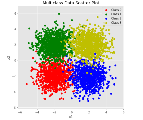
    plt.show()

plot_multiclass_decision_boundary(lambda x: predict_multiclass(params, x), X, y)

Further Evaluation

from numpy.random import RandomState

plt.style.use('ggplot')
#plt.style.use(['dark_background'])
#plt.style.use('classic')

RNG = RandomState(42)
# Construct an example multiclass dataset
n_events = 1000
spread=1
class_0 = RNG.multivariate_normal(
    [-2, -2], np.diag([spread, spread]), n_events)
class_1 = RNG.multivariate_normal(
    [-2, 2], np.diag([spread, spread]), n_events)
class_2 = RNG.multivariate_normal(
    [2, -2], np.diag([spread, spread]), n_events)
class_3 = RNG.multivariate_normal(
    [2, 2], np.diag([spread, spread]), n_events)

X_test = np.concatenate([class_0, class_1, class_2, class_3])
y_test = np.ones(X_test.shape[0])
w = RNG.randint(1, 10, n_events * 4)
y_test[:1000]*= 0
y_test[2000:3000]*= 2
y_test[3000:4000]*= 3
permute = RNG.permutation(y_test.shape[0])
X_test = X_test[permute]
y_test = y_test[permute]

plot_multiclass_scatted_data(X_test, y_test)

output:

plot_multiclass_decision_boundary(lambda x: predict_multiclass(params, x), X_test, y_test)

output:

XX: (1000, 1000), XX.ravel: (1000000,)
yy: (1000, 1000), yy.ravel: (1000000,)
np.c concated shape(1000000, 2) as Predidction_data
Prediction Data: Before Transpose (1000000, 2)
Prediction Data: After Transpose (2, 1000000)
Z: Before Reshape (1000000,)
Z: After Reshape (1000, 1000)
4000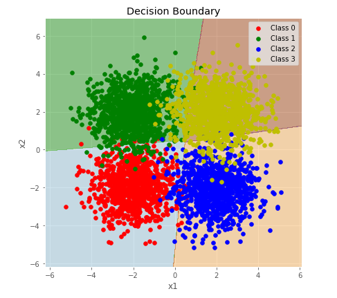

To get any other help you can contact us at:

realcode4you@gmail.com

or comment in below comment section and get instant help with an affordable price.